Estimating Mean Using Central Limit Theorem

Estimating Mean Using Central Limit Theorem

According to the central limit theorem, the mean of a sample of data will be closer to the mean of the overall population in question, as the sample size increases, notwithstanding the actual distribution of the data. In other words, the data is accurate whether the distribution is normal or aberrant.

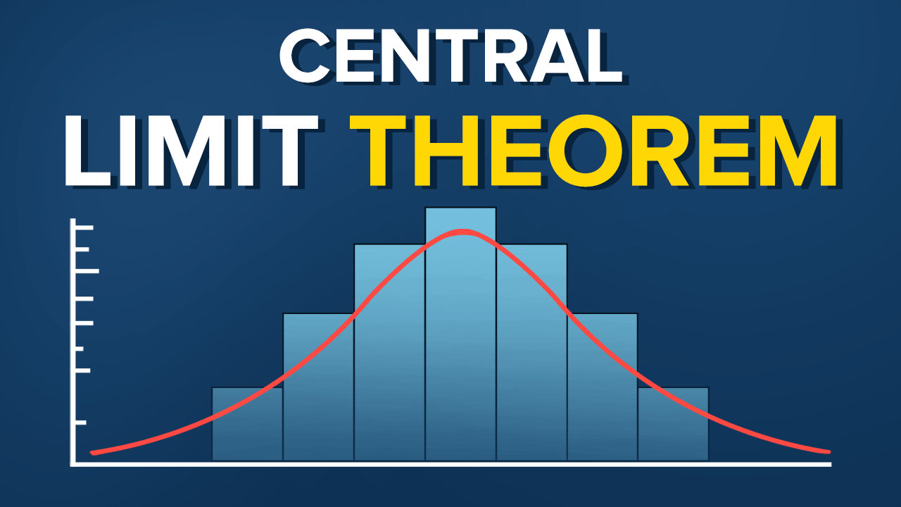
As a general rule, sample sizes equal to or greater than 30 are deemed sufficient for the CLT to hold, meaning that the distribution of the sample means is fairly normally distributed. Therefore, the more samples one takes, the more the graphed results take the shape of a normal distribution.

Central Limit Theorem exhibits a phenomenon where the average of the sample means and standard deviations equal the population mean and standard deviation, which is extremely useful in accurately predicting the characteristics of populations.

The central limit theorem is one of the most important results in probability theory. It states that, under certain conditions, the sum of a large number of random variables is approximately normal. Here, we state a version of the that applies to i.i.d. random variables.

Suppose that $X_{1},X_{2},.....X_{N}$ are i.i.d. random variables with expected values $EX_{i} = \mu < \infty$ and variance $var\left ( X_{i} \right )= \sigma ^{2}< \infty$ .

the sample mean

$\bar{X}= \frac{X_{1}+X_{2}+....+X_{n}}{n}$

has mean $E\bar{X}=\mu$

and $var\left ( \bar{X} \right )=\frac{\sigma ^{2}}{n}$ variance .

Thus, the normalized random variable

$Z_{n} =\frac{\bar{X}-\mu}{\sigma /\sqrt{n}}=\frac{X_{1}+X_{2}+.....+X_{n}-n\mu }{\sqrt{n}\sigma }$

has mean EZ_n=0 and variance Var(Zn)=1. The central limit theorem states that the CDF of Z_n converges to the standard normal CDF.

Impact on Machine Learning

The central limit theorem has important implications in applied machine learning.

The theorem does inform the solution to linear algorithms such as linear regression, but not exotic methods like artificial neural networks that are solved using numerical optimization methods. Instead, we must use experiments to observe and record the behavior of the algorithms and use statistical methods to interpret their results.

Let’s look at two important examples.

Significance Tests

In order to make inferences about the skill of a model compared to the skill of another model, we must use tools such as statistical significance tests.

These tools estimate the likelihood that the two samples of model skill scores were drawn from the same or a different unknown underlying distribution of model skill scores. If it looks like the samples were drawn from the same population, then no difference between the models skill is assumed, and any actual differences are due to statistical noise.

The ability to make inference claims like this is due to the central limit theorem and our knowledge of the Gaussian distribution and how likely the two sample means are to be a part of the same Gaussian distribution of sample means.

Confidence Intervals

Once we have trained a final model, we may wish to make an inference about how skillful the model is expected to be in practice.

The presentation of this uncertainty is called a confidence interval.

We can develop multiple independent (or close to independent) evaluations of a model accuracy to result in a population of candidate skill estimates. The mean of these skill estimates will be an estimate (with error) of the true underlying estimate of the model skill on the problem.

With knowledge that the sample mean will be a part of a Gaussian distribution from the central limit theorem, we can use knowledge of the Gaussian distribution to estimate the likelihood of the sample mean based on the sample size and calculate an interval of desired confidence around the skill of the model.